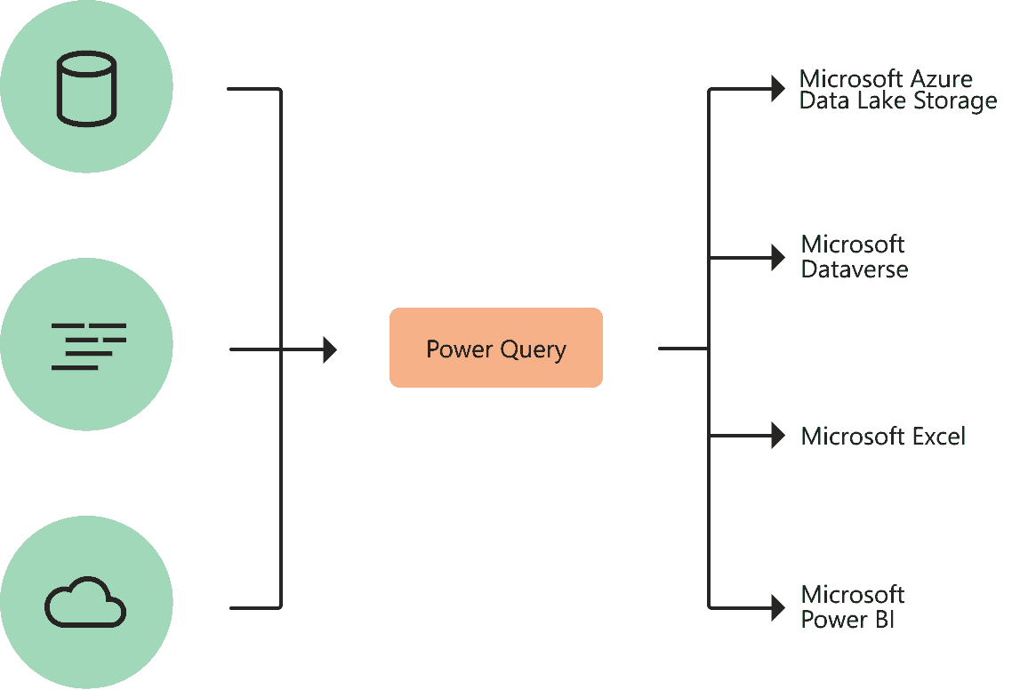
PowerQuery is a powerful tool in Excel that allows you to import, clean, and analyze data from various sources. One of the key features of PowerQuery is its ability to refresh data automatically, which can be particularly useful when you want to update subheadings based on the data in your source. In this article, we will explore how to use Power Query to achieve this and provide step-by-step instructions for implementing automatic data updates.

Getting Started with Power Query
1. Open Excel and ensure that the Data tab is visible. If it is not, you can enable it by going to File > Options > Customize Ribbon and checking the Data box.
2. Click on the Data tab and select “From Table/Range” to open the Power Query editor.
3. In the Power Query editor, you will see a list of steps that have been applied to your data. These steps represent the transformations and actions performed on the data.
Refreshing Data in Power Query
To refresh data in Power Query, you can either click on the “Refresh” button in the Power Query toolbar or go to the “Home” tab and click on “Refresh”. This will update the data in your query and apply any changes you have made to the source data.
Automating Data Updates with Subheadings
To automatically update subheadings based on the data in your source, you can use a combination of Power Query functions and formulas. Here’s a step-by-step guide:
1. In the Power Query editor, identify the column or column that contains the values you want to use for the subheadings.
2. Create a new column in the Power Query editor to store the subheading values. You can do this by clicking on the “Add Column” button in the Power Query toolbar.
3. In the new column, use a formula or function to extract the subheading values from the source data. For example, if your source data is in column A and you want to create subheadings based on the values in column B, you can use the following formula:
=IF(ISNUMBER(MID(A1, 1, LEN(A1) – 1)), “Subheading ” & MID(A1, 1, LEN(A1) – 1), “”)
This formula checks if the first character of the value in column A is a number, and if so, it extracts the subheading value. If the first character is not a number, it returns an empty string.
4. Once you have created the subheading column, you can rename it and move it to the desired location in the Power Query editor.
5. In the final step, click on the “Close & Load” button in the Power Query toolbar to apply the changes and load the data back into Excel.

Refreshing Power Query Automatically
To refresh Power Query automatically when the source data changes, you can use a macro. Here’s how to do it:
1. Press `ALT + F11` to open the Visual Basic Editor.
2. Click on “Insert” > “Module” to create a new macro module.
3. In the macro module, write a function that updates the subheadings based on the source data. You can use a similar formula as in the previous step, but this time, wrap it in a function and call it from the macro.
4. Create a Worksheet Change event in the macro to trigger the function whenever the source data changes.
5. Close the Visual Basic Editor.
Now, whenever the source data changes, the macro will automatically update the subheadings in your Excel sheet.
Conclusion
Using Power Query, you can automate data updates with subheadings in Excel. By following the steps in this article, you can create a dynamic and interactive data environment that updates subheadings based on the data in your source. This can be particularly useful for creating interactive dashboards, reports, and data visualizations that need to be updated regularly.


